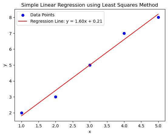
Regression: Simple Linear Regression

Regression : Regression is a statistical method used for predicting continuous outcome ( dependent variable ) based on one or more input features ( independent variables ).

Purpose : To identify the relationship between variables, understand patterns and make future predictions.

e.g. Predict someone’s weight based on their height.

Goal : Given a training set comprising $N$ observations {$x_n$}, where $n=1,2,3 … N$ together with corresponding target values {$t_n$}, where $n=1,2,3 … N$ the goal is to predict the value of $t$ for a new value of $x$.

Common Regression Algorithms :

1. Simple Linear Regression : Relationship between two variables
2. Multiple Linear Regression : Relationship between one dependent and multiple independent variables
3. Polynomial Regression : Extension of linear regression by adding Polynomial terms
4. Ridge and Lasso Regression : Regularization Techniques.
5. Multivariate adaptive regression splines

Simple Linear Regression

Let’s take an example of the number of hours a student studied and the score obtained by the student. What will be the exam score for a student who studied for 5 hours?

Study Hours	Exam Scores
2 hrs	12
4 hrs	16
8 hrs	28
16 hrs	62

In this example we have only one feature or the input is only one dimensional and we are trying to find a linear relation between them. Thus it’s an example of simple linear regression.

Equation of the Regression Line :

---

$y=mx+c$

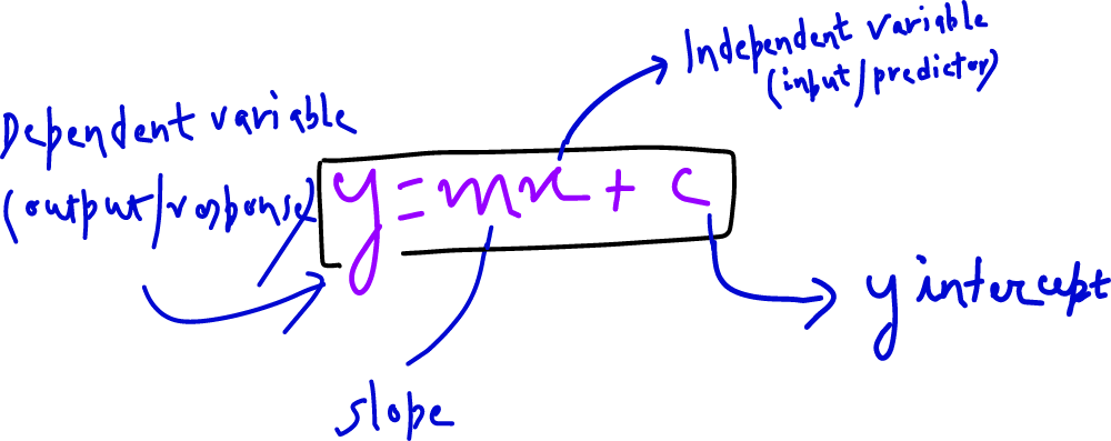
Given the assumption that there is a linear relationship b/w the independent and dependent variable, how to find the values of $m$ and $c$, so let’s look at one of the methods to solve this

Cost Function (Error Function) :

To measure the accuracy of the regression line, we use a cost function (also called the loss function). The most common cost function is “Mean Square Error (MSE)” which calculates the average of the squared differences between actual and predicted values.

Sum of Squares Error (SSE) :

$SSE = \sum_{i=1}^{N} (y_i - \hat{y_i})^2$

where $y_i$ : actual value of the dependent variable

$\hat{y_i}$ : predicted values of the dependent variables

$N$ : the total number of data points

Actual Values	Predicted Values
5	6
4	4
2	1

$SSE = (5-6)^2 + (4-4)^2 + (2-1)^2 = 1+0+1 = 2$

Mean Square Error (MSE) :

$MSE = \frac{\sum_{i=1}^{N} (y_i - \hat{y_i})^2}{N}$

where N : number of datapoints in consideration.

Thus for the above example $MSE = \frac{(5-6)^2 + (4-4)^2 + (2-1)^2}{3} = \frac{2}{3}$

Now using the least square method we will try to minimize the cost function.

Least Squares Method

Let’s say for $i^{th}$ data point, the predicted value is $\hat{y_i} = mx_i + c$. Then the error (residual) for the $i^{th}$ data point:

$Error = y_i - \hat{y_i} = y_i - (mx_i + c)$

The SSE of the model is :

$SSE (m, c) = \sum_{i=1}^{N} (y_i - \hat{y_i})^2$

$= \sum_{i=1}^{N}(y_i - (mx_i + c))^2$

To find the value of m,c that minimizes the cost function. We have to take Partial derivative w.r.t ‘m’ and Partial derivative w.r.t ‘c’:

Partial Derivative w.r.t m :

$\frac{\partial SSE}{\partial m} = \frac{\partial }{\partial m} (\sum_{i=1}^{N} (y_i - mx_i -c)^2 )$

$= \sum_{i=1}^{N} -2\times(y_i - mx_i - c)\times x_i$

making $\frac{\partial SSE}{\partial m} = 0$

$=> \sum_{i=1}^{N} -2\times(y_i - mx_i - c)\times x_i = 0$

$\sum x_i y_i = m \times \sum (x_i)^2 + c \times \sum x_i$ --------------> eqn 1

Similarly Partial Derivative w.r.t c :

$\frac{\partial SSE}{\partial c} = \frac{\partial }{\partial c} (\sum_{i=1}^{N} (y_i - mx_i -c)^2 )$

$= \sum_{i=1}^{N} 2\times(y_i - mx_i - c)\times (-1)$

making $\frac{\partial SSE}{\partial c} = 0$

$\sum_{i=1}^{N} y_i = m \times \sum_{i=1}^{N} x_i + c \times \sum_{i=1}^{N} 1$

$=> \sum y_i = m \times \sum x_i + N \times c$ -----------------–> eqn 2

Thus $c = \frac{\sum y_i - m \times \sum x_i}{N}$

Now substituting this value in equation 1, we can get

$m = \frac{\sum x_i \times \sum y_i - N \times \sum x_i \times y_i}{(\sum x_i)^2 - N \times \sum x_i }$

or $m = \frac{N \times \sum x_i \times \sum y_i - \times \sum x_i \times y_i}{N \times (\sum x_i)^2 - \times \sum x_i }$

Now, Let’s take an example set of datapoints and see how to work with least square method.

e.g. Consider a dataset of points as below, find the best fit line y = mx + c using the least square method.

x	y
1	2
2	3
3	5
4	7
5	8

Solution :

As per formula above,

or $m = \frac{N \times \sum x_i \times \sum y_i - \times \sum x_i \times y_i}{N \times (\sum x_i)^2 - \times \sum x_i }$

$c = \frac{\sum y_i - m \times \sum x_i}{N}$

x	y	x.y	$x^2$
1	2	2	1
2	3	6	4
3	5	15	9
4	7	28	16
5	8	40	25
$\sum x_i = 15$	$\sum y_i = 25$	$\sum x_i y_i= 91$	$\sum (x_i)^2 = 55$

Thus $m = \frac{(5 \times 91) - (15 \times 25) }{(5 \times 55) - (15)^2}$

$= \frac{80}{50} = 1.6$

similarly $c = \frac{25 - 1.6 \times 15}{5}$

$c = 0.2$

Thus the best fit using least square method is $y = 1.6x + 0.2$

Now, lets look at some python code to implement the same

# Import necessary libraries
import numpy as np
import matplotlib.pyplot as plt

# Given data points
x = np.array([1, 2, 3, 4, 5])
y = np.array([2, 3, 5, 7, 8])

# Number of data points
n = len(x)

# Calculate sums needed for least squares method
sum_x = np.sum(x)
sum_y = np.sum(y)
sum_xy = np.sum(x * y)
sum_x_squared = np.sum(x ** 2)

# Calculate slope (m) and intercept (c)
m = (n * sum_xy - sum_x * sum_y) / (n * sum_x_squared - sum_x ** 2)
c = (sum_y - m * sum_x) / n

# Print the calculated values of m and c
print(f"Slope (m): {m}")
print(f"Intercept (c): {c}")

# Plotting the data points
plt.scatter(x, y, color='blue', label='Data Points')

# Plotting the regression line
plt.plot(x, m * x + c, color='red', label=f'Regression Line: y = {m:.2f}x + {c:.2f}')

# Labeling the axes
plt.xlabel('x')
plt.ylabel('y')
plt.title('Simple Linear Regression using Least Squares Method')

# Adding a legend
plt.legend()

# Display the plot
plt.show()

Slope (m): 1.6
Intercept (c): 0.2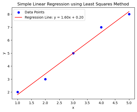

Gradient Descent Method for Simple Linear Regression

Instead of directly substituting the derivative to zero, we make small changes to the hyperparameters (m, c i.e parameters which we tune for the model) to get optimal value of m and c.

Step 1 : Take an initial value of hyperparameters m and c.

Step 2 : Iteratively adjust the parameters m and c in the direction that reduces cost.

$m_{new} = m_{old} - \alpha \frac{\partial MSE}{\partial m}$

$c_{new} = c_{old} - \alpha \frac{\partial MSE}{\partial c}$

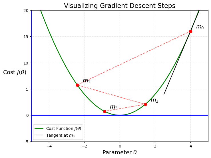
Gradient of $J (\theta) \mid_{\theta = \theta_{0}} => \frac{\partial J (\theta)}{\partial \theta} \mid_{\theta = \theta_{0}}$

Thus if gradient of $J(\theta)$ at $m_0$ > 0 then we m should decrease further for an optimal solution. Similarly if $m_0 \< 0$ then m should increase.

Where $\alpha$ is another hyperparameter which is used to manage at what rate the decrease in m or c should happen and is also called the learning rate

As we have already seen,

$MSE = \frac{\sum_{i=1}^{N} (y_i - \hat{y_i})^2}{N}$

thus, $\frac{\partial MSE}{\partial m} = \frac{-2}{N} \sum_{i=1}^{N} x_i (y_i - (mx_i + c))$

thus, $\frac{\partial MSE}{\partial c} = \frac{-2}{N} \sum_{i=1}^{N} (y_i - (mx_i + c))$

Let’s look at this in code,

# Import necessary libraries
import numpy as np
import matplotlib.pyplot as plt

# Given data points
x = np.array([1, 2, 3, 4, 5])
y = np.array([2, 3, 5, 7, 8])

# Number of data points
n = len(x)

# Hyperparameters
learning_rate = 0.05
epochs = 200  # Number of iterations

# Initialize m (slope) and c (intercept) to zero
m = 0
c = 0

# Store history of m and c for plotting
m_history = [m]
c_history = [c]

# Gradient Descent Function
for epoch in range(epochs):
    y_pred = m * x + c  # Predicted values
    
    # Calculate the gradients
    dm = (-2/n) * np.sum(x * (y - y_pred))
    dc = (-2/n) * np.sum(y - y_pred)
    
    # Update parameters
    m -= learning_rate * dm
    c -= learning_rate * dc
    
    # Store values for plotting
    m_history.append(m)
    c_history.append(c)
    
    # Print values every 20 epochs
    if (epoch + 1) % 20 == 0:
        print(f"Epoch {epoch + 1}: m = {m:.4f}, c = {c:.4f}")

# Plotting the data points
plt.scatter(x, y, color='blue', label='Data Points')

# Plotting the regression line
plt.plot(x, m * x + c, color='red', label=f'Regression Line: y = {m:.2f}x + {c:.2f}')

# Labeling the axes
plt.xlabel('x')
plt.ylabel('y')
plt.title('Simple Linear Regression using Least Squares Method')

# Adding a legend
plt.legend()

# Display the plot
plt.show()

Epoch 20: m = 1.5555, c = 0.3606
Epoch 40: m = 1.5684, c = 0.3142
Epoch 60: m = 1.5775, c = 0.2812
Epoch 80: m = 1.5840, c = 0.2577
Epoch 100: m = 1.5886, c = 0.2411
Epoch 120: m = 1.5919, c = 0.2292
Epoch 140: m = 1.5943, c = 0.2208
Epoch 160: m = 1.5959, c = 0.2148
Epoch 180: m = 1.5971, c = 0.2105
Epoch 200: m = 1.5979, c = 0.2075